Integrated GeoFactor --

Part and Tolerance Relationship Analysis

New Feature in 3DCS Version 7.7 - See all the new features in 3DCS V7.7

Why this is helpful -- Understand how the relationship between parts in an assembly magnify your tolerances without the need for an add-on module.

What Is GeoFactor?

Understanding the Geometric Effect (hence G-Factor) provides a better understanding of the behavior of your product, and why it may be at risk of failure despite appearances.

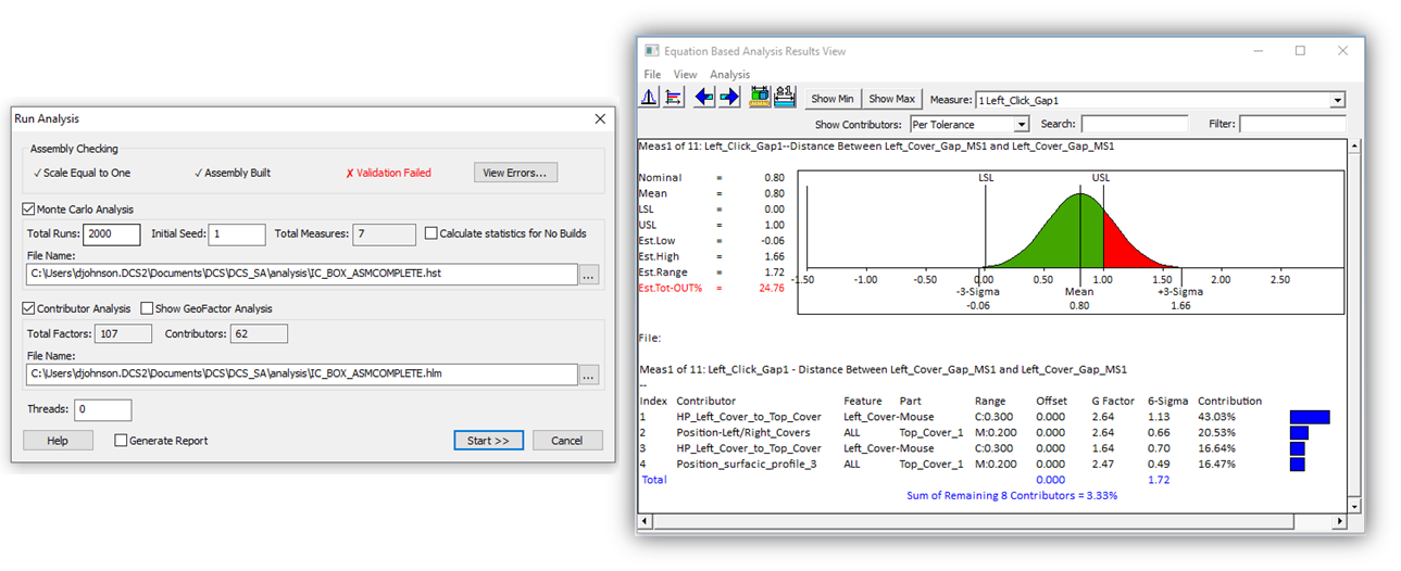
Sensitivity calculates the effect of each tolerance on a measurement. It calculates the tolerance contribution based on geometric effect, tolerance's range, bonus tolerance and Distribution of Range.

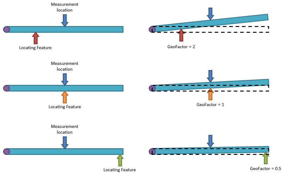
To quantify the geometric effect, GeoFactor provides a G Factor value for each contributor. If a contributor has a G Factor with an absolute value less than 1, then the variation of the contributor is mitigated by the part geometry at the measurement location. If a contributor has a G Factor with an absolute value greater than 1, then the variation of the contributor is amplified by the part geometry at the measurement location. Basically, the G Factor number is the scalar of each contributor on the measurement.

The following illustration is a simple example of G Factor. A beam is pinned on the left side and the vertical height of the center of the beam is measured. Three different locating schemes are used. The same small deviation is applied to the locating feature for each scheme. The difference of the three schemes is due to the position of the locating feature. The farther the locating feature is from the pinned end, the less variation in the measurement. This is represented by smaller G Factors.

G Factor Illustration

Sensitivity takes the input range of an individual tolerance and calculates the Sigma value for that range based on the distribution type.

Sigma*G Factor*6 = Effective 6-Sigma

Then all the Effective 6-Sigma's are added up via a Root Sum Squares calculation. This is how the overall 6 Sigma variation is predicted by Sensitivity.

Depending on the Linearity of the model, the 6 Sigma value will match the 6STD value from the Simulation results. The Curve Fit data (Estimated Type and Estimated Range) from the Simulation Analysis indicates if the results have a Normal distribution, and therefore will also be comparable with the Sensitivity results. Sigma for a Uniform distribution is different then sigma for a Normal distribution, therefore a different result will be generated. For example, changing from a Normal distribution to a Uniform distribution will result in a larger sigma value, changing the Sensitivity results.