How Does Simulation Based Sensitivity Work? Learn some here, and then join us for a webinar to see for yourself!
August 31st - Simulation Based Sensitivity
-- Improve sensitivity accuracy on complex models and get more detailed results - New analysis feature coming for 3DCS Advanced Analyzer and Optimizer (AAO) Add-on Module
Click to Join the Webinar (It's Free, promise)
Simulation Based Sensitivity is a new advanced analysis tool coming out for 3DCS Advanced Analyzer and Optimizer Add-on (AAO) for all versions of 3DCS software. In the following explanations, remember that the current version of AAO contains GeoFactor calculations, and uses the same calculation methods as GeoFactor.
Simulation Based Sensitivity is the next stage in the advancement of 3DCS analysis. We can now see into 3DCS model behavior in ways not possible before. Besides the usual HLM lists, we now gain insight into multivariate interactions between inputs and their effects on output mean shift.
Designed experiments gain a high level of accuracy because of Simulation Based regression. Simulation Based Sensitivity presents all this rich information to the user in several different viewing flavors - variance, mean shift, geometric coefficients, and more.
Currently with the GeoFactor and AAO tools we refer to G Factor (or just Factor) values and 6-Sigma values.

In Simulation Based Sensitivity (SBS), we are currently using the terms Coefficients and Amounts for similar calculated results.
In a linear model without interactions (between the contributors, e.g. bonus tolerance) and all normal distributions, GeoFactor/AAO and SBS will produce the same results for each pair of terms.
Otherwise, the results will be different because the terms represent similar but not identical calculations and values.
In GeoFactor, the G Factor is the coefficient in the equation:
Measure Current Value = G Factor * Current Tolerance Deviation.
Thus, a G Factor of -1.2 means that if the tolerance deviates to 0.1 mm, the measure current value will change by -0.12 mm.
The G Factor is directly calculated from two measure results: those with the tolerance deviated by plus and minus the gradient step. (Floats and Circular/Diametric Position tolerances are a little more complicated.)

In GeoFactor, we assume the contributors don't interact (except with a couple of known, coded adjustments, e.g. bonus tolerance.) We also assume the G Factor is the slope of a straight line defining the change in the measure value for any tolerance deviation value.
Therefore, GeoFactor calculates the assumed 6-Sigma measure result from each tolerance range using the G Factor and some adjustments (e.g. scaling by 3^0.5 if a Uniform distribution is used.) This is the expected Measure 6STD result if the model is run with only this contributor active.
Since the contributors are assumed to be independent, a Total (measure 6-sigma) value can be calculated by RSSing each contributor's 6-Sigma value. This value needs to be confirmed with a simulation run.
The Percent Contributions are calculated from these values.
Then, if a contributor's range is changed, the 6-Sigma and Percent Contribution values can be immediately updated. Results have to be confirmed with a simulation run.
So, a lot of assumptions are required for GeoFactor/AAO (and HLM) analysis.
SBS eliminates many or most of these assumptions by using simulation results. Instead of using two measure results for each contributor, it uses thousands.
So SBS give much more detailed and meaningful results with a trade-off of dramatically longer analysis times.
(Which is why we have two new features coming out at the same time to dramatically reduce your analysis times! These features, available in version 7.4.1.0, include the new multi-core processing and cloud computing. Learn about these in September at our next webinar in the series)

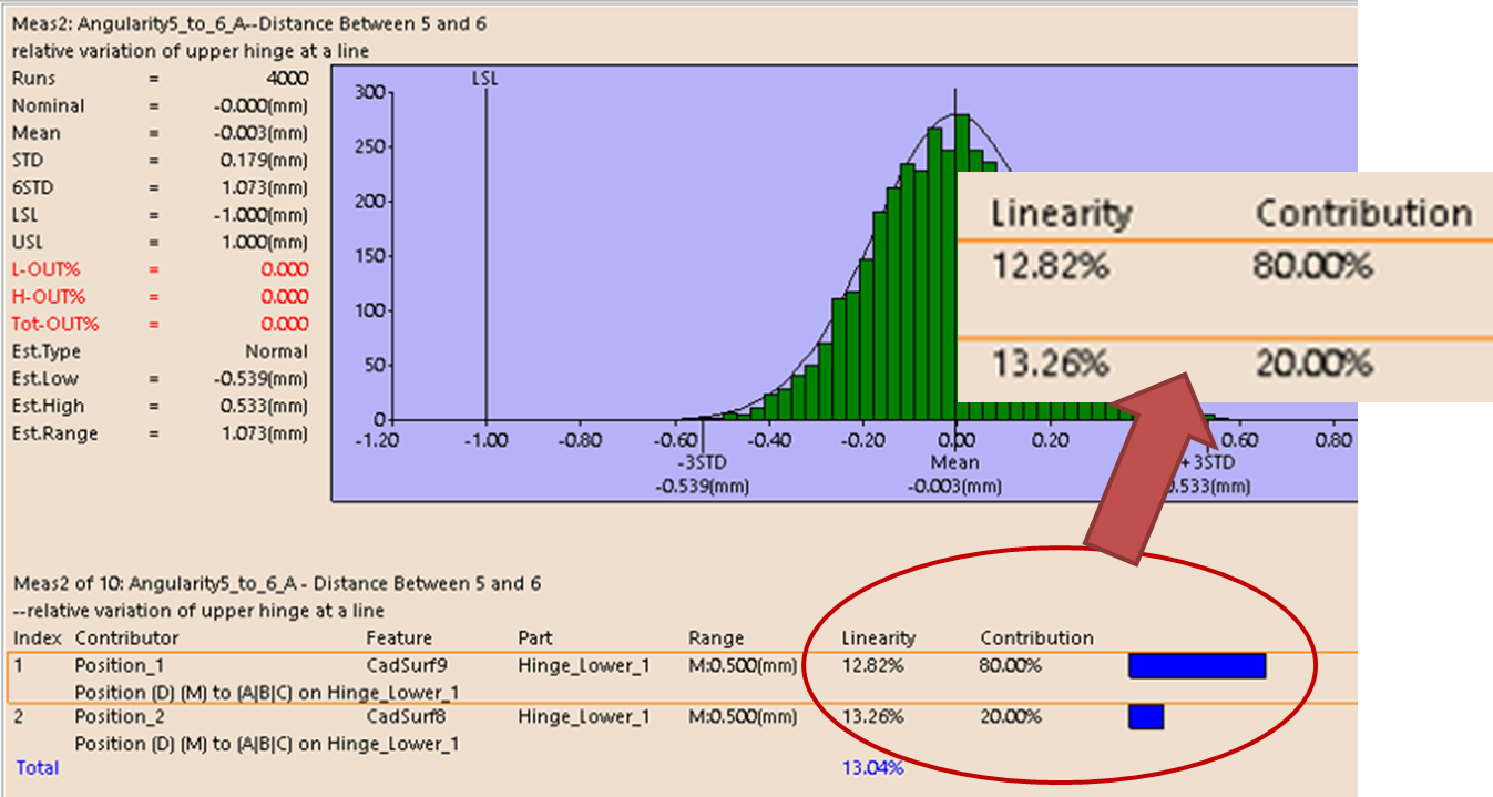
This analysis window shows an example of poor linearity, and would be a good example of when to use Simulation Based Sensitivity (SBS)
To calculate the Coefficient of a particular contributor, SBS runs a simulation with the range of that contributor set to x and all other ranges set to 0.000001 (not zero to preserve the random number stream.) The measure 6STD for a particular measure will be an Amount y. Therefore, the Coefficient for the contributor-measure pair will be y/x. Since neither the contributor range nor the measure 6STD can be negative, the coefficients for the direct contributors will always be positive (there may be an exception I haven't found yet.)
Therefore, Coefficients include everything happening in the model. A linear tolerance with a range of 1 mm uniform distributed that has a G Factor of 1 would have a Coefficient of 1.732. Both the Amount and the 6-Sigma values would be 1.732 mm.

To reiterate, the G Factor relates a particular tolerance deviation to a particular measure current value, while a Coefficient relates a particular tolerance range to a particular measure 6STD.
To calculate the Coefficient of the interaction of a particular set of contributors, SBS runs simulations with each combination of the contributors with their ranges set to x or 0.000001. It then uses the measure 6STD from each simulation to calculate the Amount of the measure 6STD from just that interaction.
So, GeoFactor/AAO calculates the G Factor first and then the 6-Sigma value, while SBS calculates the Amount first (from the simulation runs) and then the Coefficient.
Because the Amount for a particular interaction of contributors involves subtracting measure results, it can and will often be negative. A negative Amount means the combined effect of the contributors decreases or mitigates the expected measure 6STD result as compared to an RSS stack. An interaction with a negative Amount will also have a negative Percent Contribution.
The Percent Contributions in SBS are calculated directly from the Amounts, so they directly reflect the simulation results. This is why they are more meaningful and reliable.
Once the SBS table is generated, the user has the option of assuming the Coefficients represent linear contributor/interaction and measure relationships. If they do, then they can change the contributor ranges and predict the new measure results. They still need to confirm the new results with a simulation run, but they are more likely to be confirmed.
Everything SBS does to predict the measure 6STD it also does to predict the measure mean results too. SBS uses the same terms (Amounts and Coefficients) for this analysis. For mean shift analysis, negative values (Amounts and Percent Contribution) indicate the mean is getting smaller or more negative. Positive values indicate the mean is increasing.
Here are some simple examples to illustrate the above. Values are rounded.
Example 1 --
For example, a simple model contains one point, one measure, and two linear tolerances. Both tolerances have ranges of 1 mm. One tolerance has a Normal distribution and the second tolerance has a Uniform distribution. Both have G Factors of 1. In this measure, the tolerances do not interact (they are completely independent.) Both HLM/AAO/GeoFactor and SBS will calculate percent contributions of 25% and 75% respectively. (the percentages are based on the variance values.)
Example 2 --
Another simple model contains two point and two linear tolerances, one on each point. Both tolerances have ranges of 1 mm and Normal distributions. Both have G Factors of 1. For a certain measure, the tolerances interact so that the measure 6STD is 2.0 mm.
AAO/GeoFactor won't measure the interaction, so it will report a Total 6-Sigma of 1.4 mm and a 50% contribution from each tolerance.
SBS will detect the two tolerances interact to amplify the measure variation so it will report a Total 6-Sigma of 2.0 mm. It will report a third contributor, the interaction between the two tolerances (the direct contributors) that adds an amount of variation equivalent to 1.4 mm. The percent contributions for the two tolerances will be 25% and 25% and the percent contribution for the interaction will be 50%. The user can see the two tolerances are more important than the univariate analysis suggests. If the user reduces the range of one of the tolerances, they will see that both it and the interaction contribution will be reduced.
For a second measure, the Nominal value is 1 mm but the Mean is 1.28 mm. SBS finds each tolerance causes a mean shift of 0.13 mm by itself and the interaction causes an additional 0.02 mm of mean shift. Therefore, the percent contributions are 46%, 46%, and 7%.
Similar calculations occur when negative values are calculated by SBS.
Example 3 --
For a third measure, the Nominal value is 0 mm. SBS finds each tolerance causes a mean shift of about 0.13 mm by itself and the interaction causes about negative 0.08 mm of mean shift. Therefore, the Mean is only 0.19 mm.
Example 4 --
For a fourth measure, when looking at the Variance matrix, the Amounts are 1 mm for each tolerance and -0.747 mm for the interaction. The RSS calculation will yield an expected measure 6STD of 1.2 mm.
That is, (1 + 1 - 0.56)^0.5
Watch the blog next week for our follow up article, "When to Use Simulation Based Sensitivity in Tolerance Analysis"
Interested in more? See for yourself how SBS works, and can be applied to your tolerance models by Brenda Quinlan, one of the key developers of the tool.
August 31st - Simulation Based Sensitivity Webinar
-- Improve sensitivity accuracy on complex models and get more detailed results - New analysis feature coming for 3DCS Advanced Analyzer and Optimizer (AAO) Add-on Module


North American Innovation Center
28064 Center Oaks Ct A, Wixom, MI 48393
Call us: +1 (248) 504 6200


No Comments Yet
Let us know what you think