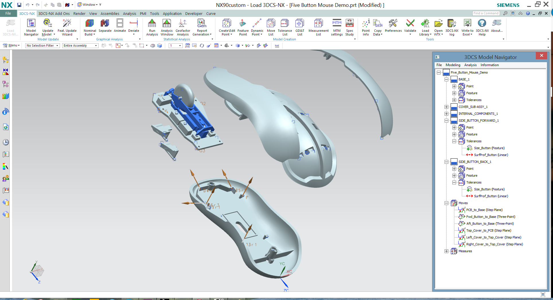
What are Some Methods of Variation Analysis?

There are a number of different methods developed to both describe variation on models and drawings, as well as analyze and control the impact of that variation.

In a typical assembly process, dimensional variation is affected by tolerances (including component and operationinduced tolerances) and operations. Tolerance Analysis is focused on tolerances and assumes operations are known. Dimensional Variation Analysis analyzes both tolerances and operations. For example, operation sequence or operation type is an analysis topic for Dimensional Variation Analysis.

What Is Vectorial Dimensioning and Tolerancing?

Vectorial Dimensioning and Tolerancing (VDT) is a different method to specify dimensions and tolerances, in contrast to Geometric Dimensioning and Tolerancing (GD&T). The concept of VDT is to use a substitute element instead of the actual element in its calculations. The substitute element is a calculated geometrical ideal feature, such as a plane, cylinder, or circle. VDT avoids ambiguity in calculating location, orientation, and form variation for a specific feature.

In VDT, a substitute element can be represented as a 7- element vector (Px, Py, Pz, θx, θy, θz, S), where (Px, Py, Pz) indicates the location, (θx, θy, θz) indicates the orientation, and S indicates the size if applicable.

Following the VDT notation, a vectorloop method assumes that real features can be accurately represented by 7- element vectors. Therefore, a much simplified method – Vector-loop Tolerance Analysis – can be utilized considering only location and orientation.

How is Discrete-Time State Space Method Used in Dimensional Variation Analysis?

A state variable is the analysis system’s internal state representation, which may not always be measurable. In the StateSpace concept, any discrete-time system can be represented as a set of algebraic equations based on state variables.

x(k+1) = A(k) x(k) + b(k)u(k) + w(k) (State Equation)

(1) y(k+1) = C(k) x(k) + d(k)u(k) + v(k) (Output Equation)

(2) Where vector x(k) is the state vector, u(k) is the input vector,

y(k) is the output vector, matrix A(k) is the system matrix,

C(k) is the output matrix, b(k) and d(k) are constant vectors,

w(k) and v(k) are system noise vectors, and k is the time sequence.

A multi-station variation model can be devised by treating k as a station index instead of a time sequence. In this case, the state vector x(k) is now a stack of feature representations;

u(k) contains variation factors at station k; and y(k) contains measurements at station k.

For example, when two planar features are concerned, a 12-element vector can be created as follows: x = (P1x, P1y, P1z, θ1x, θ1y, θ1z, P1x, P2y, P2z, θ2x, θ2y, θ2z) Where (P1x, P1y, P1z) and (θ1x, θ1y, θ1z) are the first feature location and orientation; (P2x, P2y, P2z) and (θ2x, θ2y, θ2z) are the second feature location and orientation respectively.

Based on the above State-Space Variation representation, a State Equation can be constructed for each station (operation). Once a State-Space Variation model is developed, the related Control Theory can be applied to variation analysis and synthesis.

For example, the observability can be used to determine the minimum number of measurements needed. The controllability can be used in optimizing variation factors, station sequence, and station type. Interestingly, a feedback control mechanism can be designed for the automation of a production process.

[For further information about Control Theory, see Chi-Tsong Chen, Analog and Digital Control System Design, Saunders College Publishing, 1993]

What is the Stream-Of-Variation Analysis?

Stream-of-Variation Analysis (SOVA) is an analysis and synthesis framework for multi-station assembly processes based on station-indexed state-space theory. A SOVA system is utilized in modeling, analysis, synthesis and control of process variation for multi-station manufacturing systems.

The SOVA process model can be summarized as follows: